2 Medical Background and Datasets
Medical research on data from clinical and epidemiological studies lays the foundation for decisions about diagnosing and treating multifactorial conditions such as diseases and disorders. Major goals are to identify long-term determinants and protective factors for an outcome of interest [3]–[5], discover subpopulations with increased disease prevalence [6]–[8], and study intervention effects by generating statistical models explaining cause-and-effect relationships [9]–[11]. Traditional medical data analysis pipelines are usually structured in a hypothesis-driven way as follows [16]:
- A medical scientist formulates a hypothesis based on observations in clinical practice or current research. Possible examples include: “How does a risk factor such as alcohol abuse affect the prevalence of a particular outcome?” or “What effect does a novel therapy have on patients with depressive symptoms?”
- A small set of relevant variables that can be controlled for confounders is selected to test this hypothesis. Variable selection may include controlling for confounders. The data necessary to test the hypothesis are then collected.
- The strength of associations between the selected variables and the outcome is assessed using regression models and statistical methods.
- Based on the results, inferential statistical calculations will be performed, and conclusions will be drawn that may support the implementation of new preventive interventions or the use of appropriate treatments in high-risk patients.
However, with the advent of big data [33] in various fields, including medicine, data volume and heterogeneity are increasing dramatically, making traditional hypothesis-driven workflows increasingly inadequate as important relationships between variables may go undetected [18]. In this thesis, we present methods that deal with different aspects of high-dimensional timestamped medical data. We validate our methods on a variety of datasets from diverse study types.
This chapter is divided into two parts. Section 2.1 provides a brief comparison of medical study types. In Section 2.2, we present the studies and the data samples for which we developed the methods proposed in this thesis.
2.1 Brief Comparison of Medical Study Types
Primary medical research can be divided into basic, clinical, and epidemiological studies [34]. The following comparison of these study types is based on the reviews of Thiese [35] and Röhrig et al. [34] if not indicated otherwise.
Basic research. Basic medical research (or experimental research) aims to improve the understanding of cellular, molecular, and physiological mechanisms of human health and disease by conducting cellular and molecular investigations, animal studies, drug and material property studies in tightly controlled laboratory environments. To study the effects of one or more variables of interest on the outcome, all other variables are usually held constant, and only the variables of interest are varied. The carefully standardized experimental conditions of basic medical studies ensure high internal validity, but these conditions often cannot be easily transferred to clinical practice without compromising the results’ generalizability.
Clinical studies. Clinical studies are generally classified into interventional (experimental) studies and non-interventional (observational) studies. The general objective of an intervention study is to compare different treatments within a patient population whose members differ as little as possible except for the treatment arm. A common example is a pharmaceutical study that aims to validate the efficacy and safety by investigating or establishing a drug’s main and side effects, absorption, metabolism, and excretion. Selection bias can be avoided by appropriate measures, in particular by randomly assigning patients to groups. Treatment may be a medication, surgery, therapeutic use of a medical device (e.g., a stent), physical therapy, acupuncture, psychosocial intervention, rehabilitation, training form, or diet. A randomized controlled trial (RCT) is considered the gold standard of study design [36]. Selection bias is minimized by (a) randomly assigning patients to treatment and control groups and (b) ensuring equal distribution of known and unknown influencing variables (confounders), such as risk factors, comorbidities, and genetic variability. RCTs are thus suitable for obtaining an unambiguous answer to a clear question concerning the (causal) efficacy of a treatment.
Non-interventional clinical trials are patient-based observational studies in which patients either receive an individually defined treatment, or all patients receive the same treatment. An example of a non-interventional design is a study investigating the regular use of drugs in therapies. Here, treatment, diagnosis, and monitoring do not follow a predefined study protocol but rather medical practice alone. Data analysis is often retrospective. Whether a study design is prospective or retrospective depends on the sequence of hypothesis generation and data collection. In prospective studies, hypothesis generation comes before data collection. First, the hypotheses to be tested are defined, e.g., regarding a new treatment procedure. Then, data are collected specifically for hypothesis testing. By first formulating testable hypotheses, it is possible to ensure that the research questions can actually be answered with the measured data. A retrospective study design means that data collection took place before the study began.
Epidemiological studies. Epidemiological studies are usually interested in the distribution and change over time of the incidence of diseases and their causes in the general population and subpopulations. Cohort studies examine individuals, some of whom do not have the health outcomes of interest at the beginning of the observation period and assess exposure status to various health-related conditions [37]. The included subjects are then followed up over time in longitudinal studies (as opposed to cross-sectional studies), where the outcomes of interest are recorded in multiple waves. With these data, researchers can establish subgroups of subjects by exposure status, sort them by exposure, and compare the incidence or prevalence of a disease among exposure categories. Longitudinal studies are further categorized into trend and panel design. In a trend study, each wave can involve a different participant sample, i.e., an individual participant is not followed over time. In contrast, a panel study investigates the same population at multiple points in time which allows to also measure intra-individual temporal changes.
2.2 Datasets Investigated in This Thesis
In this section, we present the datasets and the associated studies investigated in this thesis, namely
- the Study of Health in Pomerania in Section 2.2.1,
- an observational therapy study on the health of tinnitus patients at baseline and after therapy in Section 2.2.2,
- a clinical experiment study on diabetic foot syndrome in Section 2.2.3, and
- a retrospective clinical study with image data on intracranial aneurysms in Section 2.2.4.
2.2.1 The Study of Health in Pomerania (SHIP)
After the reunification of Germany, it was found that life expectancy was significantly lower in the East than in the West [38]. Furthermore, there were regional differences within the new states, with the lowest life expectancy found in the Northeast [38], [39]. To find causal risk factors of mortality and other conditions in the northeastern German population, the Community Medicine Research Center in Greifswald established the Study of Health in Pomerania (SHIP) [12], a longitudinal epidemiological study of two independent cohorts in northeastern Germany. SHIP seeks to describe a broad spectrum of health conditions rather than focusing on a specific target disease [12]. In particular, major study objectives include investigations of the prevalence of common diseases and their risk factors, the correlation and interaction between risk factors and diseases, the progression from subclinical to manifest diseases, the identification of subpopulations with increased health risk, the prediction of concomitant diseases, as well as the usage and costs of medical service.
Cohort inclusion criteria were age from 20 to 79 years, main residency in the study region, and German nationality. Participants of SHIP underwent an extensive, recurring (ca. every 5 to 6 years) examination program that encompasses personal interviews, body measurements, exercise electrocardiogram, laboratory analysis, ultrasound examinations, and whole-body magnetic resonance tomography (MRT). Baseline examinations for the first cohort were performed between 1997 and 2001 (SHIP-0, N = 4308). Follow-up examinations were carried out in 2002-2006 (SHIP-1, n = 3300), 2008-2012 (SHIP-2, n = 2333), 2014 - 2016 (SHIP-3, n = 1718) and since 2019 (SHIP-4). Figure 2.1 illustrates participant response and age distribution of show-ups across study waves. Baseline information for a second, independent cohort (SHIP-Trend-0, N = 4420) was collected between 2008 and 2012, and a follow-up was conducted between 2016 and 2019. Major strengths of SHIP are a high level of quality assurance, standardized examination protocols, and a high cohort representativeness.
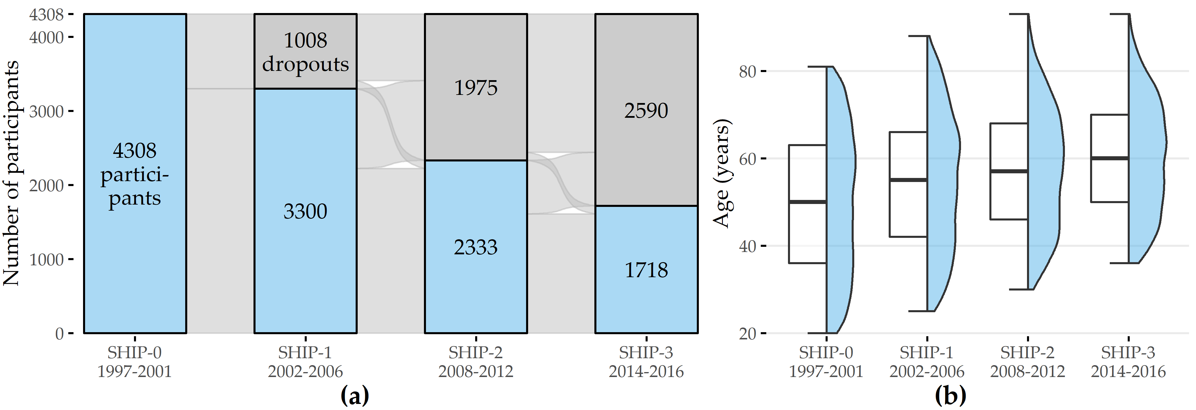
Figure 2.1: Participation response and age distribution of show-ups across SHIP study waves. (a) Change in the number of show-ups and non-respondents relative to the cohort size across waves. (b) Age distribution of show-ups for each wave.
The examination program changed across waves. For example, MRT was not performed until SHIP-2; liver ultrasound was performed in SHIP-0 and SHIP-2 but not in SHIP-1; dermatologic examinations were performed in SHIP-1 and SHIP-2 but not in SHIP-0.
Our analyses focus on the disorder hepatic steatosis, also known as “fatty liver,” characterized by a high accumulation of fat in the liver, occurring in approximately 30% of all adults [12], [40]. Risk factors include alcohol abuse, obesity, metabolic syndrome, and diabetes [41]. Liver biopsy is considered the diagnostic gold standard [42] but is associated with intermediate risk for the patient. Non-invasive diagnostic techniques include MRI, CT, and ultrasound. Because hepatic steatosis is usually asymptomatic, it often goes undetected, which can develop into more serious diseases, such as steatohepatitis, cirrhosis, hepatocellular carcinoma, or even liver failure [42].
We used SHIP data subsets to validate the methods presented in Chapters 3, 4, 6, and 9.
2.2.2 The Charité Tinnitus Patients Observational Therapy Study Dataset (CHA)
Tinnitus is the perception of a phantom sound in the absence of an external sound source. It is a complex, multifactorially caused and maintained phenomenon and is estimated to affect 10% to 15% of the adult population [43]. The associated annual economic burden is 19.4 billion USD in the United States [44] and 6.8 billion EUR in the Netherlands alone [45]. Clinical evaluation of tinnitus is challenging due to patient heterogeneity in tinnitus perception (laterality, pitch, noise characteristics, frequency, duration, chronicity), risk factors (including hearing loss, temporomandibular joint disorder, aging), comorbidities (including hyperacusis, depression, sleep disorders), perceived distress, and treatment response [46]. These differences complicate the identification of an appropriate and effective treatment modality. Currently, there is no treatment gold standard: sound therapy (masking), informational counseling (minimal contact education), cognitive behavioral therapy, and tinnitus retraining have been shown to be effective for some patients, but there is also evidence that not all patients benefit equally from these forms of treatment [47]–[51]. Due to the heterogeneous nature of the tinnitus symptom and the unclear evidence base regarding its treatment and management, identification of patient subgroups is critical to stratify individual pathophysiology and treatment pathways [52]–[54].
The “Charité tinnitus patients observational therapy study dataset” (CHA) includes self-report data from 4103 tinnitus patients treated at the Tinnitus Center of Charité Universitätsmedizin Berlin, Germany, between January 2011 and October 2015. All patients were 18 years of age or older and had suffered from tinnitus for at least 3 months. Exclusion criteria were the presence of acute psychotic illness or addiction, deafness, and insufficient knowledge of the German language. Treatment included a 7-day multimodal program with intensive and daily informational counseling, detailed ear-nose-throat psychological diagnosis, cognitive behavioral therapy interventions, hearing exercises, progressive muscle relaxation, and physical therapy. At baseline (T0; before the start of therapy) and after treatment (T1), patients were asked to complete several self-report questionnaires. These questionnaires were selected to obtain a comprehensive assessment of tinnitus, including tinnitus-related distress and the psychosomatic background of tinnitus with anxiety, depression, the general quality of life, and experienced physical impairments.
| Name | Scope | |F| | |
|---|---|---|---|
| 1 | ACSA: Anamnestic Comparative Self-Assessment [55] | Quality of life | 1 |
| 2 | ADSL: General Depression Scale [56], [57] | Depressive symptoms | 22 |
| 3 | BI: Berlin Complaint Inventory [58] | General well-being, autonomic nervous system, pain and emotionality | 29 |
| 4 | BSF: Berlin Mood Questionnaire [59] | Mood | 36 |
| 5 | ISR: ICD-10 Symptom Rating [60] | Mental disorders | 36 |
| 6 | PHQK: (Short-form) Patient Health Questionnaire [61] | Symptoms of depression and anxiety | 16 |
| 7 | PSQ: Perceived Stress Questionnaire [62] | Stress | 35 |
| 8 | SES: Pain Perception Scale [63] | Pain | 29 |
| 9 | SSKAL: Visual Analog Scales Pain | Pain impairment, frequency and intensity | 3 |
| 10 | SF8: Short Form 8 Health Survey [64] | Health-related quality of life | 18 |
| 11 | SOZK: A socio-demographics questionnaire [65] | Gender, partnership status, education, employment status, among others | 27 |
| 12 | SWOP: Self-Efficacy- Optimism-Pessimism Scale questionnaire [66] | Self efficacy, optimism, pessimism | 12 |
| 13 | TINSKAL: Visual analogue scales | Tinnitus loudness, frequency and distress | 3 |
| 14 | TLQ: Tinnitus Localization and Quality questionnaire [67] | Location (left, right, bilateral, entire head) and sound of tinnitus | 8 |
| 15 | TQ: Tinnitus Questionnaire (German version) [68] | Tinnitus-related distress and tinnitus severity | 60 |
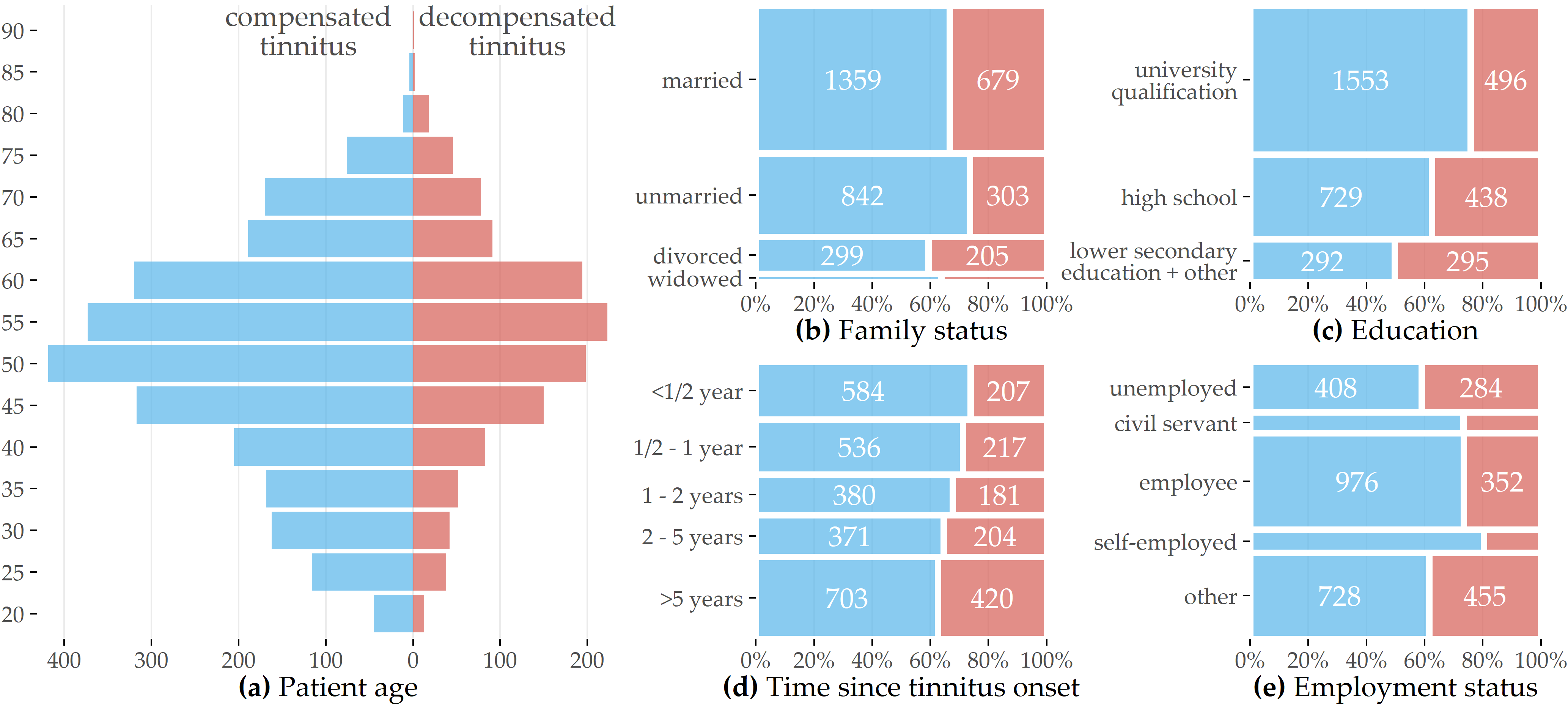
Figure 2.2: Patient demographics (CHA). Overview of patient demographics by degree of tinnitus distress measured before therapy commencement.
Table 2.1 provides an overview of all questionnaires used in our analyses. Most questionnaires contain multiple-choice items with answers on a Likert scale. For example, the “Tinnitus Questionnaire” [68] (TQ) contains 52 statements, such as “I am unable to enjoy listening to music because of the noises.” and respondents can give 3 possible answers: “not true” (coded as 0), “partly true” (1), and “true” (2). Some questionnaires also include aggregate variables called “subscales” and “total scores.” For example, the TQ total score (TQ_distress) is calculated as the sum of 40 item values, with 2 items used twice [68], resulting in a range of values from 0 to 84, with higher values representing higher tinnitus-related distress. The cutoff value 46 [68] is used to distinguish between compensated (0-46) and decompensated (47-84) tinnitus. Furthermore, the average time to answer an item was recorded for each questionnaire. Figure 2.2 provides a graphical representation of demographic data for 3803 (92.7%) patients with complete data for the socio-demographics questionnaire [65] (SOZK) and TQ score.
We used the CHA dataset to validate the methods developed in Chapters 5, 8, and 9.
2.2.3 The Diabetic Foot Clinical Experiment Study (DIAB)
Diabetic foot syndrome is an umbrella term for foot-related problems in diabetic patients. Up to one in four diabetes patients will develop a foot ulcer during their lifetime [69], with many at risk of amputations in the next four years [70]. More than 85% of foot amputations are due to foot ulcers [71], [72]. The rate of foot amputations in diabetes patients is estimated to be 17-40 times higher than in the general population [73]. DFS patients are predisposed to peripheral sensory neuropathy, which results, for example, in patients being unaware of the temperature of their feet or the pressure applied to them. Affected individuals may even injure themselves without realizing it. Excessive plantar pressures can exacerbate tissue destruction and increase the lifetime risk of foot ulceration [74]. However, understanding of the pathomechanisms underlying tissue destruction in the absence of trauma is limited.
At the university hospital of Magdeburg, Germany, an experimental study with 31 healthy volunteers and 30 diabetes patients diagnosed with severe polyneuropathy was conducted to quantify pressure- and posture-dependent changes of plantar temperatures as surrogate of tissue perfusion. For this purpose, plantar pressure and temperature changes in the feet were recorded during extended episodes of standing. Custom-made shoe insoles [75] equipped with eight temperature sensors and eight pressure sensors at preselected positions were used for data acquisition (Figure 2.3 (a)). The insoles were positioned into closed protective shoes specifically developed for diabetes patients. Within such shoes, the temperature increases over time due to exchange with the person’s body temperature and is also affected by the environmental temperature. To closely monitor the in-shoe temperature changes, one sensor was placed at the bottom of the insole without contact to the feet, which was denoted “ambient temperature sensor.”
![Positions of pressure- and temperature sensors on insole and temporal, pressure-dependent temperature change. (a) Sensor positioning on the insole in relation to foot placement. (b) Thermographic infrared images showing a healthy subject in a seated position with no pressure applied to the feet (before) and after placement of a 20 kg weight on both thighs. The measured temperature ranged from 29°C (blue) to 34°C (red). A time-dependent temperature decrease was observed predominantly in the forefoot region, visualized by yellow color during pressure application. A rapid temperature increase was noted within 1 min after pressure relief. MTB: metatarsal bone. The figure is adapted from [31].](figures/02-df-infrared-sole-sensor-positions.png)
Figure 2.3: Positions of pressure- and temperature sensors on insole and temporal, pressure-dependent temperature change. (a) Sensor positioning on the insole in relation to foot placement. (b) Thermographic infrared images showing a healthy subject in a seated position with no pressure applied to the feet (before) and after placement of a 20 kg weight on both thighs. The measured temperature ranged from 29°C (blue) to 34°C (red). A time-dependent temperature decrease was observed predominantly in the forefoot region, visualized by yellow color during pressure application. A rapid temperature increase was noted within 1 min after pressure relief. MTB: metatarsal bone. The figure is adapted from [31].
Data collection began immediately after the shoes were put on. Participants were asked to follow a predefined sequence of actions, i.e., alternating between standing (stance episode) and sitting (pause). A session consisted of 6 stance episodes lasting 5, 10, 20, 5, 10, and 20 minutes, respectively, separated by pause episodes lasting 5 minutes each. Participants were instructed to apply equal pressure to both feet while standing. Participants did not receive immediate feedback on the actual application of pressure during the sessions, but they were verbally encouraged by the study nurses to maintain pressure while standing without releasing it. In the seated position, participants were instructed to release pressure for 5 minutes while maintaining contact with the insole. Participants were explicitly asked to adhere to these instructions, i.e., not to release pressure during a standing episode temporarily. The study protocol further included that the measurements were performed twice, once at room temperature of approximately 22°C and once outdoors at an ambient temperature of approximately 16°C. The two measurements were performed on two independent days.
The thermographic images in Figure 2.3 (b) visualize exemplary changes in plantar temperature in a healthy subject in a sitting position before pressure application (1), after placing a 20 kg weight on the front of the thigh (2-6), and after removing the additional weight (7-8). During pressure application, a gradual temporal decrease in temperature was noted predominantly in the forefoot. After pressure relief, a rapid temperature increase was observed within 1 min.
We used the DIAB dataset to validate the methods developed in Chapter 7.
2.2.4 The Intracranial Aneurysm Angiography Image Dataset (ANEUR)
Intracranial aneurysms are pathologic dilations of the intracranial vessel wall, often in the form of a dilation. They bear a risk of rupture, leading to subarachnoidal hemorrhages with often fatal consequences for the patient. Since treatment can also cause severe complications, extensive studies were conducted to assess the patient-individual rupture risk based on various parameters, including aneurysm symptomatology, size, location, and patient age and sex [76]. Further studies identified parameters, such as aspect ratio, undulation index, and nonsphericity index, to be statistically significant with respect to aneurysm rupture status [77], [78]. However, although these studies allow for retrospective analysis, the clinician needs further guidance if an asymptomatic aneurysm (as an accidental finding) was detected and the rupture risk should be determined.
We developed methods for the retrospective “Intracranial Aneurysm Angiography Image Dataset” (ANEUR) comprising 3D rotational angiography data from 74 patients (age: 33-85 years, 17 male and 57 female patients) of the university hospital of Magdeburg, Germany, adding up to a total of 100 intracranial aneurysms. We identified two primary goals for this dataset: (i) build models that can accurately predict rupture status based on morphological parameters only, and (ii) assess the importance of these parameters to the models with optimal accuracy.
Motivated by the results of Baharoglu et al. [79], who found differences between sidewall and bifurcation aneurysms (cf. Figure 2.4) in terms of the relationship of several morphological parameters and rupture status, we learn different models for the subset of sidewall aneurysms (9 (37.5%) of 24 ruptured) and the subset of bifurcation aneurysms (29 (46.8%) of 62 ruptured). Additionally, we run experiments on a combined group (43 of 100 ruptured) containing 14 additional samples that could not be clearly determined to be either sidewall or bifurcation aneurysms.
![Sidewall and bifurcation aneurysms. Illustration of an aneurysm at the side of the parent vessel wall (left) and an aneurysm at a vessel bifurcation (right). The figure is adapted from [32].](figures/02-aneur-sw-bf.png)
Figure 2.4: Sidewall and bifurcation aneurysms. Illustration of an aneurysm at the side of the parent vessel wall (left) and an aneurysm at a vessel bifurcation (right). The figure is adapted from [32].
We used the ANEUR dataset to validate the methods developed in Chapter 8.