6 Constructing Evolution Features to Capture Change over Time
Brief Chapter Summary
We propose a framework to extract “evolution features” from timestamped medical data, which describe the study participants’ change over time. We show that exploiting these novel features improves classification performance by validating our workflow on the SHIP data for the target variable hepatic steatosis.
This chapter is partly based on:
Uli Niemann, Tommy Hielscher, Myra Spiliopoulou, Henry Völzke, and Jens-Peter Kühn. “Can we classify the participants of a longitudinal epidemiological study from their previous evolution?” In: Computer-Based Medical Systems (CBMS). 2015, pp. 121-126. DOI: 10.1109/CBMS.2015.12.
Medical studies with a longitudinal design collect participant data from questionnaires, medical examinations, laboratory analyses, and imaging repeatedly over time [12]–[14]. Hidden temporal information could be made explicit by constructing features that describe the subjects’ change over time. However, there is a lack of applicable methods for timestamped data with a tiny (< 5) number of moments. We present a framework addressing this shortcoming and demonstrate that augmenting the feature space with so-called evolution features increases classification performance and yields understandable descriptors of change worthy of further investigation.
Section 6.1 describes work related to the construction of temporal representations in medical data. Section 6.2 introduces the notation and problem formulation. Section 6.3 presents our evolution feature framework, including a full workflow that encompasses steps to extract evolution features, dealing with class imbalance, and feature selection. Section 6.4 describe the evaluation setup. We report on our results in Section 6.5 and present evolution features found to be important for class separation in Section 6.6. We conclude this chapter in Section 6.7.
6.1 Motivation and Comparison to Related Work
Epidemiological studies serve as a basis for the identification of risk factors associated with a medical condition [3]–[5]. Machine learning is still relatively little used in epidemiology, mainly due to the hypothesis-driven nature of their research. However, examples of machine learning applications are the identification of health failure subtypes [169] and the discovery of factors (including biomarkers) that modulate a medical outcome [170], [171]. In longitudinal cohort studies, measurements are performed in multiple study waves; hence researchers obtain access to sequences of recordings. In the context of machine learning, extracting and leveraging the inherent temporal information from these sequences may increase model performance and, thus, the understanding of the medical condition of interest.
From a technical point of view, classification problems on timestamped data can be very different. They can be broadly summarized into three categories:
- Each instance (patient, study participant) has a label at each time point \(t\). The goal is to assign the instance’s label at \(t\) + 1. Typically, this is a data stream classification problem [172], [173].
- Each instance is associated with only one label for the all time points. Typically, this is a timeseries classification problem [174], [175].
- There are no labels but the time point of an event is to be predicted. This problem is concerned with event prediction [176]–[178].
Our classification problem falls under (a), but we cannot use the advances of stream classification because we our data is unlabeled except for the last time point and our stream of three time points is tiny.
In clinical applications, temporal information is often exploited, predominantly for the analysis of patient records. For example, Pechenizkiy et al. [179] analyzed streams of recordings to predict rehospitalization because of heart failure events during remote patient management. Sun et al. [180] computed the similarity between streams of patients from patient monitoring data. Combi et al. [181] reported on streams of life signals, particularly on the temporal analysis of the timestamped medical records of hospital patients.
However, participants of an epidemiological, population-based study are not hospital patients – they are a random sample of the studied population, often with a skewed class distribution. In a longitudinal study of this kind, recordings for the same cohort member are made at each moment. Hielscher et al. [182] presented a feature engineering approach to extract temporal information from multiple but few patient recordings in a longitudinal epidemiological study. First, for each assessment, clusters of feature-value sequences associated with the target variable are found. Afterward, original and sequence features are used in conjunction for classification. Hielscher et al. [182] showed that classification performance increases when features with temporal information are incorporated into the feature space. Instead of modeling the individual change of measurement values, our approach involves deriving multivariate change descriptors.
Patient evolution with clustering was studied by Siddiqui et al. [183]. They proposed a method that predicts patient evolution from timestamped data by clustering them on similarity and predicting cluster movement in the multi-dimensional space. However, the patient data considered in [183] are labeled at each moment.
Our workflow combines labeled and unlabeled timestamped data from a longitudinal study to improve classification performance on skewed data. As the target variable, we study the multi-factorial disorder hepatic steatosis (fatty liver) on a sample of participants from the longitudinal population-based “Study of Health in Pomerania” (SHIP) [12], recall Section 2.2.1. For the SHIP cohort, the assessments (interviews, medical tests, etc.) were recorded in several moments (SHIP-0, SHIP-1, etc.), that are ca. 5 years apart. Temporal information is often used when analyzing patient data in a hospital, but there the time granularity is different. For example, in an intensive care unit, timestamped data are collected at a fast pace, i.e., every minute or even every second. In contrast, the participants of a longitudinal epidemiological study are monitored for months or even years. Hence, measurements of the same assessment in an epidemiological dataset are few and possibly far apart. The large period between two consecutive recordings complicates applying methods designed for data that arrive with a higher frequency. For example, a participant may exhibit alcohol abuse or become pregnant, stop smoking and start again, take antibiotics that affect the liver, or experience other lifestyle changes that turn the medical recordings taken five years ago irrelevant for learning the participant’s current health state. Another patient may have no lifestyle changes and no illnesses, so their past data reflect only aging.
A further challenge is that the label is unavailable for several waves. A reliable estimate of the fat accumulation in the liver was computed from magnetic resonance tomography images. In SHIP-0, MRT was unavailable. Instead, liver fat accumulation was derived from ultrasound – a procedure with lower clinical accuracy. In SHIP-1, the calculation was omitted altogether. Consequently, for a given SHIP participant, the class label is available in SHIP-2, no label in SHIP-1, and a partially reliable indicator in SHIP-0. Since hepatic steatosis is a reversible disorder, label imputation – using a growth model [184] – is not possible; participant evolution must be learned with only one moment with labeled data.
We address these challenges as follows. First, we group study participants at each moment on similarity, thus building clusters of cohort members with similar recordings at one of the three moments. Then, we connect the clusters across time, thus capturing each cluster’s transition from one study wave to the next. These transitions reflect the evolution of subpopulations, not individuals. Hence, next to the single labeled recording per cohort participant, we also exploit the earlier, unlabeled recordings, the description of the cluster they are assigned to, and information on how the clusters evolve. We show that this new, augmented dataset, combining labeled and unlabeled data on individuals and subpopulations, improves classification and delivers additional insights on some factors associated with hepatic steatosis.
6.2 Problem Formulation
We now provide some basic symbols and essential functions for our classification problem, summarized in Table 6.1.
| Term | Description |
|---|---|
| \(x\) | a study participant from cohort \(X\) |
| \(t\) | a study moment, one of \(\{1,\ldots, T\}\) |
| \(f\) | a feature from the set of all features \(F\) |
| \(v(x,f,t)\) | the value of \(x\) for feature \(f\) at moment \(t\) |
| \(obs(x,F,t)\) | all measurements for \(x\) at \(t\), i.e., \(\{v(x,f,t)|\forall f\in{}F\}\) |
| \(label(x,t)\) | the class label of \(x\) at moment \(t\) |
| \(Z(t)\) | all observations at \(t\), i.e., \(\{obs(x,F,t)| \forall x \in X\}\) |
| \(c(x,t)\) | cluster membership of \(x\) at \(t\); if \(x\) is an outlier at \(t\), then \(c(x,t)\) is NULL |
| \(d(x,z,t)\) | distance between \(x\) and \(z\) at \(t\) (cf. Eq. (6.1)) |
| \(kNN(x,k,t)\) | the set of k nearest neighbors of \(x\) at \(t\) |
| \(centr(x,t)\) | centroid of \(c(x,t)\) |
Our longitudinal study comprises data for a participant \(x\in X\) for every feature \(f\in F\) and every time point \(t\in \{1,\ldots, T\}\) (also referred to as moment). The (single) value of \(x\) for feature \(f\) at moment \(t\) is denoted as \(v(x,f,t)\); the set of all values for \(x\) at \(t\), i.e., \(\{v(x,f,t)|\forall f\in{}F\}\), is denoted as \(obs(x,F,t)\). For some participant, \(v(\cdot)\) is NULL, i.e., there may be missing values. Our goal is to to predict the class label of \(x\) at moment \(T\), i.e., \(label(x,T)\) by using data from all observations in all previous moments \(t\in\{1\ldots T-1\}\). The class label of each participant is unavailable except for \(t=T\). We model this prediction task as conventional classification problem. We aim to improve classification performance by expanding the feature space with change descriptors, the so-called evolution features, presented next.
6.3 Evolution Features
We leverage latent temporal information of a longitudinal cohort study dataset by extracting informative features based on the individual change of participants and the transition of their respective clusters over time. For this purpose, we exploit the similarity among participants at each moment as a surrogate to the labels which are not available in the first two moments, assuming that similar participants evolve similarly. We call these new features “evolution features”. Our approach is illustrated in Figure 6.1 (a). We monitor the individual change of participants across the study waves, trace the clusters’ change separately, extract new features (from labeled and unlabeled data) and augment the original data space with our new descriptors of change. The complete classification workflow is depicted in Figure 6.1 (b).
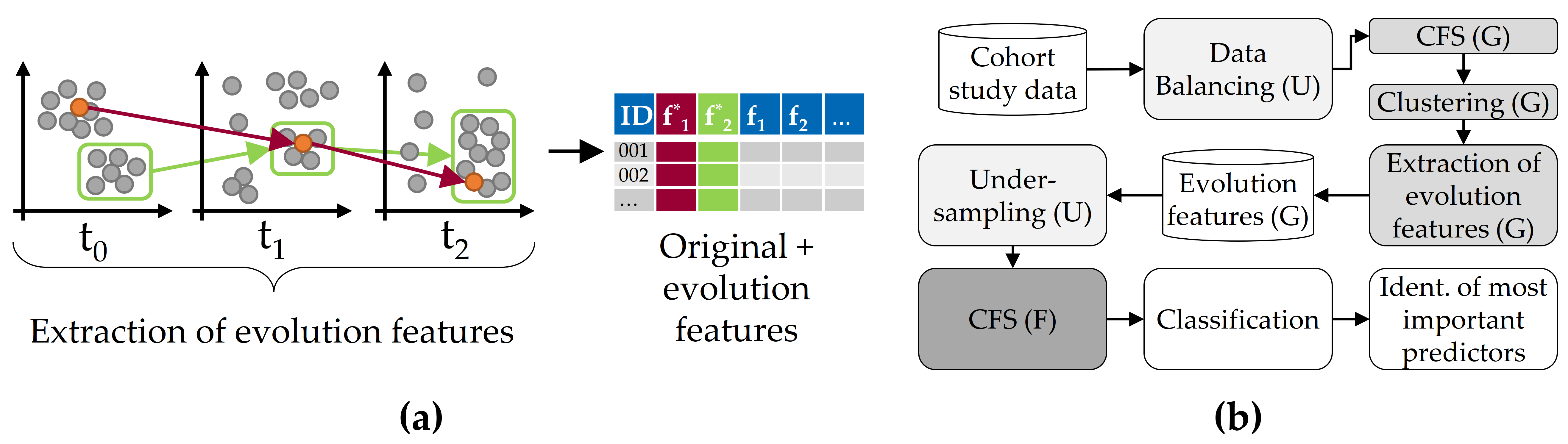
Figure 6.1: Concept of evolution feature extraction for classification performance improvement. (a) Clustering of longitudinal cohort data and subsequent generation of evolution features from the change of individuals (red) and whole clusters (green). (b) Overview of the classification workflow.
In the following, we describe the clustering of study participants (Section 6.3.1), the generation of evolution features (Section 6.3.2), and our feature selection strategy to extract a subset of informative features as input for classification (Section 6.3.3), while dealing with class imbalance by undersampling the majority class.
6.3.1 Clustering
For clustering, we prefer density-based clustering over partitional algorithms (like k-means) because our data contain extreme cases, the clusters may be arbitrarily shaped and of different sizes, and we cannot determine their number in advance. At each moment \(t\), we run the DBSCAN [185] algorithm to cluster the set \(Z(t)\) of recordings of all cohort members observed at \(t\). For participant \(x\), \(v(x,f,t)\) denotes the value of \(x\) for feature \(f\in\) feature-set \(F\) at \(t\), and \(obs(x,F,t)\) the set of all feature recordings for \(x\) at \(t\) (cf. notation in Table 6.1).
Distance function. For the distance between participants \(x,z\) at \(t\), we use the adjusted heterogeneous Euclidean overlap metric [182], [186], which weights the difference between two values \(x,z\) for feature \(f\) by the feature’s information gain \(G(f)\), scaled to the largest observed value \(G^*\), defined as: \[\begin{equation} d(x,z,t)=\sqrt{\sum_{f \in F} \left(\frac{G(f)}{G^*}\cdot \delta\left(v(x,f,t),v(z,f,t)\right)\right)^2}. \tag{6.1} \end{equation}\] For continuous features, \(\delta(a,b)\) is the min-max-scaled difference between the values \(a,b\), i.e., \((a-b)/(\max(f)-\min(f))\). For nominal features, \(\delta(a,b)\) is 0 if \(a=b\), and 1 otherwise.
DBSCAN Parameter setting. DBSCAN relies on two parameters: the radius \(eps\) of the neighborhood around a data point, and the minimum number \(minPts\) of neighbors for a point to be a core point. We use the “elbow” heuristic of Ester et al. [185], which determines a suitable \(eps\) value for a given \(minPts\) value, illustrated in Figure 6.2. More specifically, we define a parameter \(k\) and compute for each \(x\in{}Z(t)\) the distance k-dist\((x,k)\) to its kth nearest neighbor. We sort these distances, draw the k-dist\((x,k)\) graph g, and span the line l connecting the smallest k-dist() value to the largest one. Then, we set \(eps\) to the k-dist value with the maximum distance between g and l.
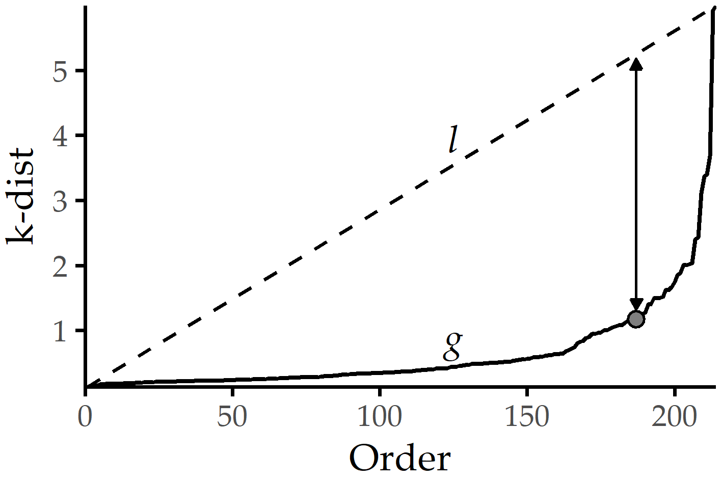
Figure 6.2: Setting \(eps\) based on the k-dist graph for a given \(minPts\). The k-dist graph g depicts the sorted distances to the points’ kth next neighbors. A suitable \(eps_{opt}\) can be identified with the maximum distance between the k-dist and the line l that connects the first and the last point of g. For DBSCAN clustering with \(minPts\) = k, \(eps_{opt}\), points with k-dist \(\leq\) \(eps_{opt}\) will become core points, else border or noise points.
6.3.2 Constructing Evolution Features
We extract information about the participants’ evolution, distinguishing among those that evolve smoothly and those that switch among clusters. We transfer this information to evolution features, thus enriching the feature space with information from the unlabeled moments. Table 6.2 describes all evolution features. They are divided into four categories: (A) features for each participant at each moment, (B) evolution features describing some aspect of change between study waves for an individual participant, (C) evolution features measuring changes between study waves concerning feature values for each participant, and (D) evolution features linked to a whole cluster.
For each cohort member \(x\) and moment \(t\), we record the cluster containing \(x\) (feature 1 in Table 6.2), (2) the distance of \(x\) to this cluster’s centroid, (3) the fraction of positively labeled participants among the k nearest neighbors of \(x\), (4) the (graph-based) cohesion [187] and (5) Silhouette coefficient [187] of \(x\), and (6) the (graph-based) separation [187] of \(x\) to cohort participants outside this cluster. We compute the difference of the cohesion, Silhouette, and separation values from \(t\) to all later moments \(\{t' \in T|t'>t\}\) (7-9), and also check how much the values of these metrics change as \(x\) moves from \(c(x,t)\) to \(c(x,t')\) (10-12). We record whether \(x\) is an outlier, i.e., a DBSCAN noise point at some moment (13). For \(t\) and \(\{t' \in T|t'>t\}\), we compute the fraction of cohort members who are in the same cluster as \(x\) in \(t\) and \(t'\) (14), and the fraction of common k nearest neighbors (15), and the change of the distance between \(x\) and its centroid at \(t\), from \(t\) to \(t'\) (16). We further record changes in the sequence of values for a feature, including real (17), absolute (18), and relative (19) differences between the values at two moments. We measure how a cluster shrinks/grows from \(t\) to \(t'\) (20), and how much its members move (on average) closer or far apart from their previous positions (21-23).
| # | Name | Description |
|---|---|---|
| (A) Features for participant \(x\) at each moment | ||
| 1 |
Cluster_t
|
Cluster ID of \(x\) at \(t\) |
| 2 |
dist_To_Centroid_t
|
Distance of \(x\) to the centroid of cluster \(c(x,t)\), denoted as \(\widehat{c(x,t)}\) |
| 3 |
fraction_Of_POS_kNN_\(k\)_t
|
Fraction of the k nearest neighbors of \(x\) at \(t\) from the positive class |
| 4-6 |
a_t := a(x,t,c(x,t))
|
\(a\) is one of {cohesion, Silhouette, separation} [187]; cohesion\(_t\) is the cohesion of \(x\) at \(t\) w.r.t. the members of \(c(x,t)\) – and similarly for silhouette and for separation |
| (B) Evolution features linked to each participant \(x\) | ||
| 7-9 |
a_Delta_t_t'
|
Difference \(a_{t} - a_{t'}\) for \(a\) as above |
| 10-12 |
a_Movement_t_t'
|
Difference \(a(x,t,c(x,t)) - a(x,t',c(x,t))\) for \(a\) as above, referring to the same cluster \(c(x,t)\) at two moments \(t,t'\); at \(t'\), \(x\in{}c(x,t')\), which does not need to be the same as \(c(x,t)\) |
| 13 |
was_becomes_Outlier_t_t'
|
Four-valued flag on whether \(x\) was outlier in both \(t, t'\), only in \(t\), only in \(t'\) or in neither\(t, t'\) |
| 14 |
same_Cluster_t_t'
|
\(c(x,t)\cap{}c(x,t')\setminus\{x\}\): set of cohort members that are in the same cluster as \(x\) in \(t\) and in \(t'\) |
| 15 |
same_kNN_\(k\)_t_t'
|
\(kNN(x,k,t)\cap{}kNN(x,k,t')\), i.e., the set of cohort members who are among the k nearest neighbors of \(x\) in both \(t\) and in \(t'\); they do not need to be in the same cluster as \(x\) |
| 16 |
shift_To_Old_Centroid_t_t'
|
Difference \(d(x,\widehat{c(x,t)},t')-(x,\widehat{c(x,t)},t)\) |
| (C) Evolution features associated with the value of each original feature \(f\) for participant \(x\) | ||
| 17-19 |
A_Diff_f_t_t'
|
Difference between \(v(x,f,t)\) and \(v(x,f,t')\) for feature \(f\), where \(A\) is either real difference, absolute difference or relative difference to \(v(x,f,t)\) |
| (D) Evolution features linked to a whole cluster \(c\) | ||
| 20 |
smaller_Cluster_Fraction_t_t'
|
Difference of the size of cluster \(c\) at \(t'\) and its size at \(t\); \(c\) is matched to the clusters of \(t\) based on member overlap |
| 21-23 |
movement_d_t_t'
|
Distance \(d\) between the locations of the members of cluster \(c\) at \(t\) and their locations at \(t'\), where \(d\) is one of Euclidean distance, HEOM distance (cf. Eq. (6.1)), Cosine similarity |
6.3.3 Extending Correlation-Based Feature Selection to Include Evolution Features
For imbalanced data, feature selection and classification are often biased in favor of the majority class [188]. Hence, before feature selection, we undersample the majority class and generate a balanced data set to select features informative with respect to all classes. We use the feature selection method of Hielscher et al. [189] as follows: we invoke correlation-based feature selection [190] (CFS), which builds up a feature set by iteratively inserting the feature that adds the most “merit” to it. The merit \(M_F\) of a feature set \(F\) is computed by calculating the information gain for each pair of features in \(F\) (lower gain corresponds to low correlation and is thus preferred) and for each feature in \(F\) towards the target variable (higher gain is better). Continuous features are first discretized with the entropy-based method of Fayyad and Irani [136]. We discretize only for feature selection; for clustering and classification, we use the original values.
As shown in Figure 6.1, we perform feature selection twice. The first time, we consider only features recorded in all moments, which is essential for evolution tracing: we can only compute distances between objects in clusters located in the same topological space. After generating the evolution features, we build up the complete set of features, also considering those not recorded in each moment. On this set, we perform feature selection again to discard unpredictive (original or evolution) features. This final feature set is then used for classification.
6.4 Evaluation Setup
We evaluate our workflow with 10-fold cross-validation on four off-the-shelf classification algorithms: random forest [191] (RF), C4.5 decision tree [192], Naïve Bayes (NB), and k-nearest neighbor (kNN).
First, we compare each algorithm’s generalization performance when used alone (baseline variant) vs. when incorporated into our workflow (workflow-enhanced variant).
Further, we study the impact of different combinations of the three workflow components undersampling (U), feature selection (F), and incorporation of generated evolution features (G).
Sensitivity (true positive rate), specificity (true negative rate), and F-measure (harmonic mean of precision and recall) serve as evaluation measures.
As shown in Table 6.3, Baseline invokes only the classification algorithm; we use the classification algorithm which achieves the highest F-measure scores.
The variant U-G performs undersampling and uses the generated evolution features for classification.
Since we undersample only for feature selection and then build the classification models on the original dataset, so U-G is identical to --G and U-- is identical to the Baseline variant, so we omit to list U-G and U-- explicitly.
The main parameter is \(k\) which is the number of neighbors of a data point: we set \(minPts\) = \(k\) and use \(k\) to derive the values of the DBSCAN parameter \(eps\) (cf. Section 6.3.1) and of the parameters for the features same_kNN_\(k\)_t_1_t_2 and fraction_Of_POS_kNN_\(k\)_t (cf. Table 6.2).
Further, the number of nearest neighbors for the k-NN classification algorithm is also set to \(k\).
We vary \(k\) to measure its impact on classification performance.
Following the findings in Chapters 3 and 4 on the differences between female and male participants with respect to the outcome, we run the experiments on the whole dataset (PartitionAll) and on the partitions of female (PartitionF) and male (PartitionM) participants.
Finally, we list the most important features found in PartitionAll and its two subsets.
| Workflow components | Under-sampling | Feature selection | Evolution features |
|---|---|---|---|
| UFG | ✓ | ✓ | ✓ |
| UF- | ✓ | ✓ | ✗ |
| -FG | ✗ | ✓ | ✓ |
| -F- | ✗ | ✓ | ✗ |
| --G | ✗ | ✗ | ✓ |
| Baseline | ✗ | ✗ | ✗ |
6.5 Results
Figure 6.3 shows sensitivity (left), specificity (center), and F-measure (right) for the simple classifiers (gray curves) and their workflow-enhanced counterparts (same line style, colored) for different k.
![Comparison of classification performance between workflow and baseline. Sensitivity (left), specificity (center) and F-measure scores (right) of different classifiers when varying the number k of neighbors to a cohort member which impacts the clustering result. For each classifier, two performance curves are shown: a colored one for the workflow-enhanced version and a gray one for the baseline counterpart. Higher values are better for all measures. The figure is adapted from [193].](figures/06-perf-wf-classifiers-palatino.png)
Figure 6.3: Comparison of classification performance between workflow and baseline. Sensitivity (left), specificity (center) and F-measure scores (right) of different classifiers when varying the number k of neighbors to a cohort member which impacts the clustering result. For each classifier, two performance curves are shown: a colored one for the workflow-enhanced version and a gray one for the baseline counterpart. Higher values are better for all measures. The figure is adapted from [193].
Overall, each workflow-enhanced variant outperforms its simple counterpart with respect to sensitivity and F-measure, and outperforms or performs slightly worse in specificity. The workflow-enhanced Naive Bayes performs best concerning sensitivity for any k and best for k = 31. Decision trees exhibit the highest F-measure, with improvements on sensitivity and F-measure compared to its simple variant, albeit specificity being slightly worse; improvements are less for large k. Random Forests benefit the most from our workflow, with an absolute improvement in F-measure of over 30% (green vs. gray “+” curves in the right part of Figure 6.3). One explanation for the relatively low sensitivity of the simple RF variant is the large number of trees (100) learned on data samples containing very few positive examples: RF could have been trapped by the many majority class examples. This result is consistent with the specificity curve (almost straight line around 95%) of simple RF, while the F-measure is slightly above 40%. Our workflow improves RF sensitivity (63%) and F-measure (65%), while specificity remains high (90%). Overall, the impact of k on the three measures is limited for all algorithms except for the workflow-enhanced and the baseline k-NN, which is naturally affected stronger by the value of k than any other algorithm. Therefore, the workflow-enhanced variants outperform their simple counterparts in terms of sensitivity and F-measure. For some algorithms, our workflow prevents overfitting to the negative class.
The results of the workflow component-specific results in Figure 6.4 show that our complete workflow UFG and the variants UF- and --G outperform the other variants in sensitivity and F-measure.
The variants -F- and -FG perform well only regarding specificity, suggesting that feature selection may not be beneficial without undersampling for datasets with class imbalance.
![Comparison of classification performance for workflow components. Sensitivity (left), specificity (center) and F-measure scores (right) for each workflow variant and the baseline using decision tree for learning. The figure is adapted from [193].](figures/06-perf-wf-components-palatino.png)
Figure 6.4: Comparison of classification performance for workflow components. Sensitivity (left), specificity (center) and F-measure scores (right) for each workflow variant and the baseline using decision tree for learning. The figure is adapted from [193].
6.6 Identification of Important Evolution Features
The performance of the workflow variants, which include feature selection, indicates that a small number of features is sufficient for class separation. Hereafter, we report on the evolution features selected for classification and appearing among the top 15 features according to information gain for each partition; we term these features “important.”
Figure 6.5 shows that for PartitionAll 3 out of these 15 features are generated evolution features.
The boxplots (a) and (c) in Figure 6.5 refer to differences between values recorded in two moments.
The feature separationDelta_g_1_2 measures the difference in cluster separation for each participant based on the cluster assignment in moment 1 and 2, and corresponds to entry #9 in Table 6.2.
Participants belonging to the positive class exhibit a higher median in separationDelta_g_1_2 than participants without the disorder, indicating that clusters harboring mostly positive participants cover larger, more sparse areas.
The feature relative_Difference_som_huef_g_0_1 (#19) quantifies the difference in a participant’s hip circumference between SHIP-0 and SHIP-1, relative to the value in SHIP-0.
On average, study participants from both classes lose weight when they grow older. Negative participants reduce more weight than positive participants (cf. Figure 6.5 (c)), which generally reflects differences in lifestyles.
The mosaic chart in Figure 6.5 (b) for feature fraction_of_Positives_kNN_1_g_2 (#3) indicates that the “nearest neighbor” of a fatty liver participant is also more likely to exhibit the disorder than it is for a participant without fatty liver.
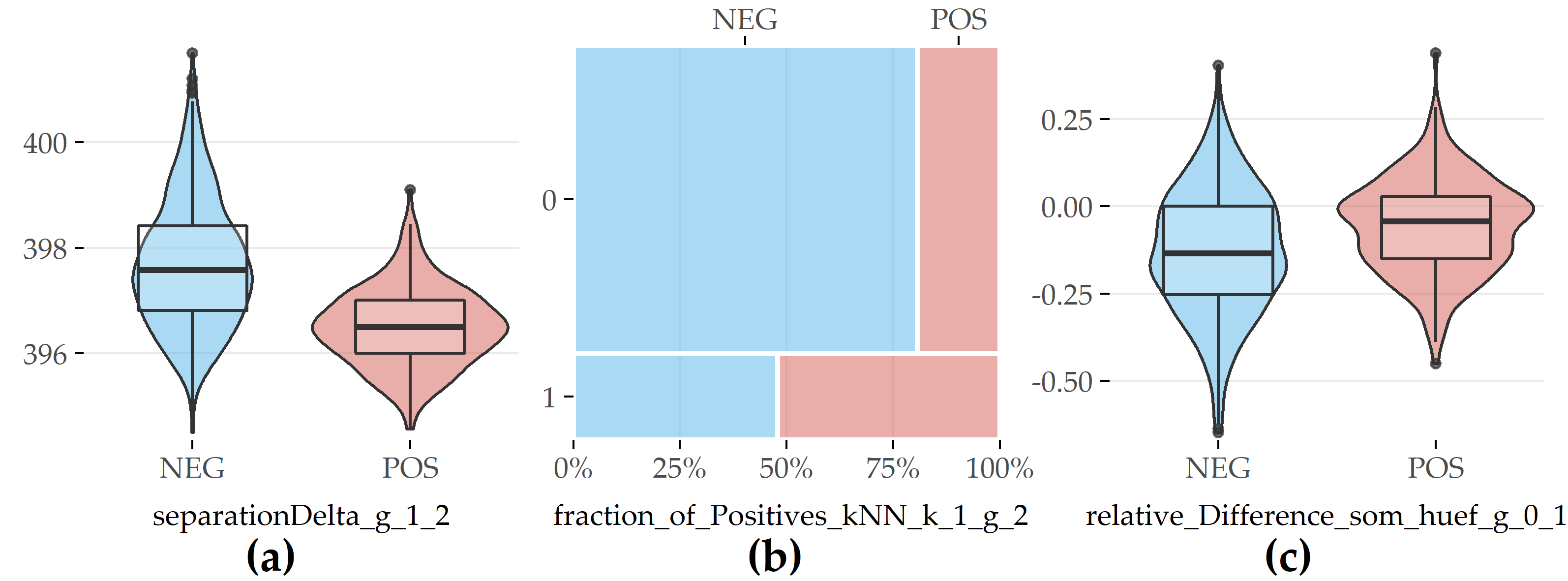
Figure 6.5: Selected evolution features with the highest contribution to class separation for PartitionAll. (a) Difference in cluster separation between SHIP-1 and SHIP-2. (b) Whether (=1) or not (=0) the nearest neighbor is of the positive class in SHIP-2. (c) Relative difference in hip circumference between SHIP-0 and SHIP-1.
For PartitionF, 5 out of the top 15 features are evolution features, cf. Figure 6.6.
Compared with female participants without the disorder, female subjects with fatty liver exhibit a larger distance to the centroid of their cluster in SHIP-1 (#2), a lower silhouette coefficient in SHIP-1 (#5), a higher difference in waist circumference between SHIP-0 and SHIP-2 (#19), and a lower relative difference in serum triglycerides concentration between SHIP-0 and SHIP-1 (#19).
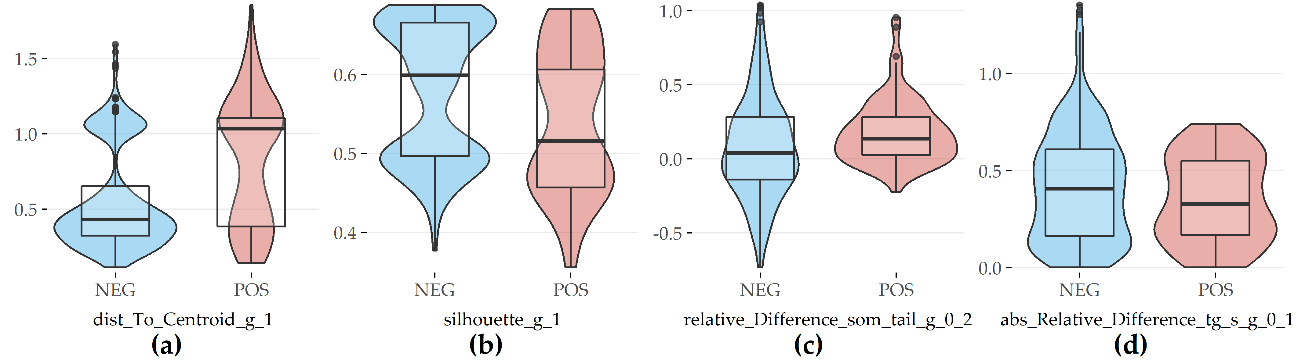
Figure 6.6: Selected evolution features with the highest contribution to class separation for PartitionF. (a) Distance to cluster centroid in SHIP-1. (b) Silhouette coefficient in SHIP-1. (c) Relative difference in waist circumference between SHIP-0 and SHIP-2. (d) Absolute value of relative difference in serum triglycerides between SHIP-0 and SHIP-1.
For PartitionM, 2 out of the top 15 features are evolution features (Figure 6.7), including the relative difference in waist circumference between SHIP-1 and SHIP-2 (#19) and difference in cluster separation between SHIP-0 and SHIP-1 (#6).
For both features, participants exhibiting the disorder have greater values.
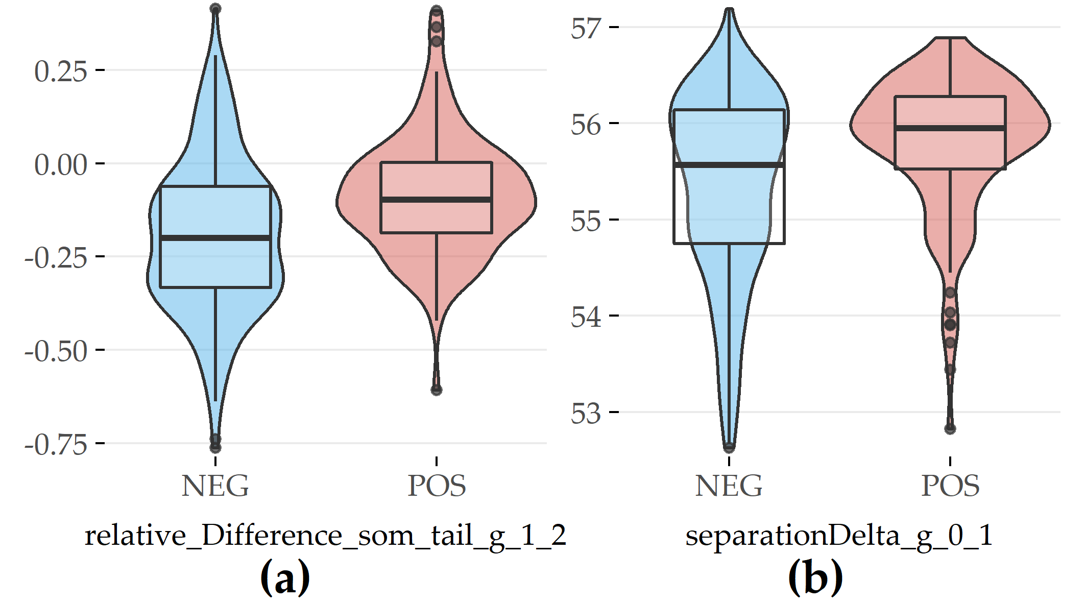
Figure 6.7: Selected evolution features with the highest contribution to class separation for PartitionM. (a) Relative difference in waist circumference between SHIP-1 and SHIP-2. (b) Difference in cluster separation between SHIP-0 and SHIP-1.
6.7 Conclusion
We have extended our set of methods for static medical data presented in Part I by proposing a workflow for the classification of longitudinal cohort study data that exploits inherent temporal information by clustering the cohort participants at each moment, linking the clusters, and tracing participant evolution over the study’s moments. We extract evolution features from the clusters and their transitions, which are added to the feature space and subsequently used for classification. The workflow improves the generalization performance with respect to sensitivity and F-measure scores. The generated evolution features contribute to this improvement, even when used alone and without undersampling the skewed data. We have shown that the change of somatographic variables’ values and cluster quality indices over time are predictive.
A limitation concerns the assessment of a feature’s importance using information gain. The additional merit a feature has towards model predictions cannot be assessed being decoupled from the actual model. Furthermore, models may incorporate complex feature interactions that are not captured or subpopulation-specific differences in feature importance. Part III addresses post-hoc model interpretation, which includes more sophisticated approaches of measuring a feature’s attribution to a model.